Introduction
XLOOKUP in Excel is one of the most powerful and modern formulas used for data lookup, reporting, and dashboard creation.
Whether you work in MIS, sales reporting, finance, HR, or data analysis, learning how to use XLOOKUP can save hours of manual work and improve reporting accuracy.
For years, professionals depended on VLOOKUP and INDEX-MATCH, but they had limitations. Today, this approach has completely transformed how we fetch and analyze data in Excel.
If you work in Excel regularly – especially in roles like MIS Executive, Data Analyst, or Sales Reporting – you already know how important lookup functions are.
I personally use this formula while preparing MIS reports and sales analysis dashboards because it reduces manual lookup errors and saves reporting time significantly.
This is not just another formula guide.
In this article, you will learn:
- Real-world XLOOKUP usage
- Advanced formula combinations
- Business-level examples
- Hands-on practice with dataset
Think of this as a mini training module, not just a blog post.
If you want to improve your reporting workflow, you should also explore our Excel Skills for Data Analysis guide where we cover advanced formulas, Pivot Tables, dashboards, and automation techniques used by professionals.
Key Takeaways
- XLOOKUP is the modern replacement for VLOOKUP.
- It supports left and right lookups.
- It works perfectly for dashboards and MIS reports.
- You can combine XLOOKUP with IF, SUM, SORT, and CONCAT.
- It helps automate reporting and reduce manual errors.
Why Use XLOOKUP
Before learning formulas, understand why it is widely used in real jobs.
Key Advantages:
- No column index number required
- Works in both directions (left & right)
- Built-in error handling
- Exact match by default
- Can return multiple values
Real Work Usage:
- Sales reporting (SKU tracking)
- MIS dashboards
- Employee data lookup
- Inventory and pricing sheets
Simply put: XLOOKUP replaces VLOOKUP in modern Excel work
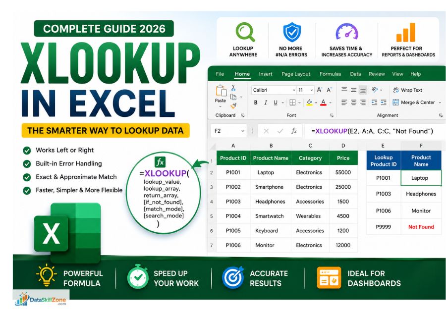
How to Use XLOOKUP in Excel
Basic Syntax:
=XLOOKUP(lookup_value, lookup_array, return_array, [if_not_found])
Example:
=XLOOKUP(A2, B:B, E:E)
Meaning:
- Find value in A2
- Search in column B
- Return result from column E
According to the Microsoft official XLOOKUP documentation, It is designed to replace older lookup formulas like VLOOKUP and HLOOKUP.
REAL Dataset (Practical Example)
Instead of small dummy data, let’s use a real business-style dataset:
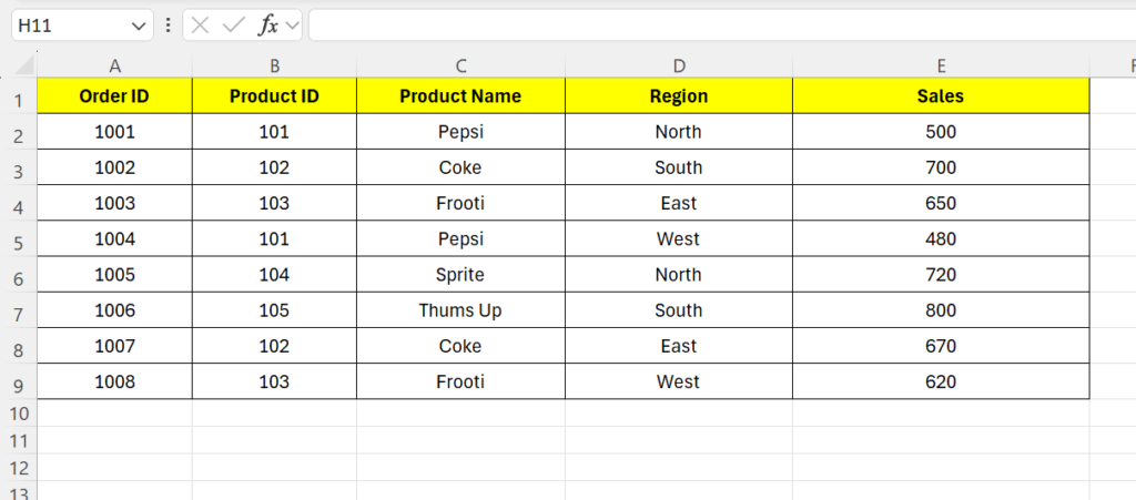
Practice sales reporting dataset
Basic XLOOKUP Example
Goal:
Find Sales using Product ID
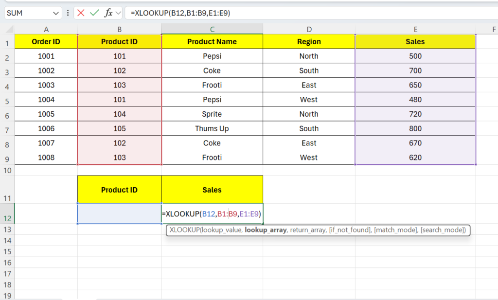
Fetch sales values dynamically using Product ID
What This Formula Does
- B12 → Product ID you want to search
- B2:B9 → Column where Excel will search
- E2:E9 → Column from where Excel returns Sales
Suppose if you entered product-id as 105, then output will be:
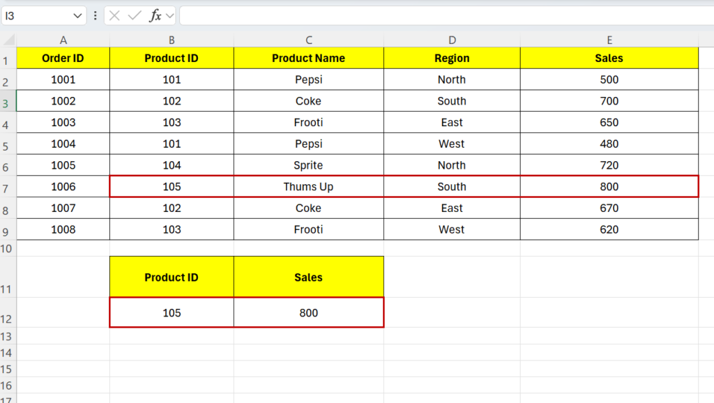
Successfully returns the matching sales value for Product ID 105
Imagine if you have 1000s of rows of sales data and your manager asks:
👉 “Can you quickly tell me the sales for a specific Product ID?”
Doing this manually would mean:
- Scrolling through large data
- Searching row by row
- High chance of mistakes
This is exactly where the lookup function saves your time.
Microsoft also provides detailed Excel learning resources through its official Excel support and training platform, where users can explore formulas, charts, Pivot Tables, and advanced Excel tools.
Advanced XLOOKUP Examples (Real Use Cases)
NESTED XLOOKUP
Now let’s take your same dataset and go one step deeper.
Scenario
Instead of directly finding Sales using Product ID, imagine this:
- You only know the Order ID
- And you want to find the Sales value
But here’s the challenge:
- Sales is not directly linked to Order ID
- You first need to find Product ID from Order ID
- Then use Product ID to get Sales
This is where Nested XLOOKUP comes into play
We will perform this in 2 steps inside one formula:
Step 1:
Find Product ID using Order ID
Step 2:
Use that Product ID to find Sales
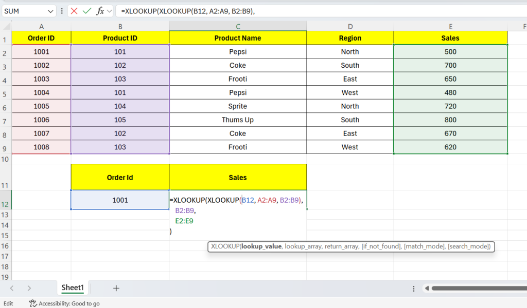
Fetch sales values dynamically from Order ID
Where:
- B12 = Order ID input
- A2:A9 = Order ID column
- B2:B9 = Product ID column
- Inner XLOOKUP returns Product ID
- Outer XLOOKUP uses that Product ID to return Sales from E2:E9
Example:
Order ID 1001 → Product ID 101 → Sales 500
So final output should be 500.
IF + XLOOKUP
This formula is used when you want to analyze the result of XLOOKUP and apply a condition.
Now Lets consider the same Example Table:
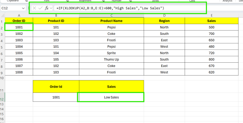
Combining to analyze sales results dynamically in Excel
In this setup, you entered Order ID = 1001 and used the formula:
=IF(XLOOKUP(A2,B:B,E:E)>600,”High Sales”,”Low Sales”)
What the Formula Does
- XLOOKUP(A2, B:B, E:E)
→ Looks for the Product ID in row A2 (linked to your data)
→ Finds the corresponding Sales value from column E - For Order ID 1001, Product ID = 101
→ Sales = 500 - IF Condition (>600)
→ Checks if Sales is greater than 600
Since 500 is less than 600
👉 Output = “Low Sales”
This formula automatically categorizes sales as High or Low based on a condition.
SUM + XLOOKUP (Combining Sales Using Order IDs)
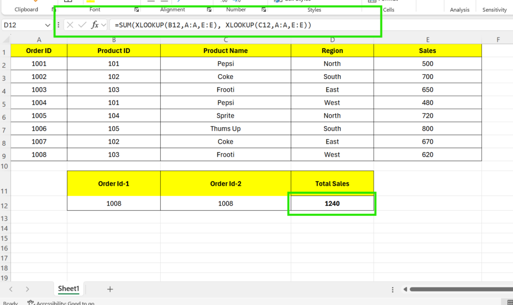
Using SUM and XLOOKUP together to combine multiple sales values dynamically in Excel
In this example, you are calculating total sales for two Order IDs.
=SUM(XLOOKUP(B12,A:A,E:E), XLOOKUP(C12,A:A,E:E))
What This Does
- B12 (Order Id-1) → 1008
- C12 (Order Id-2) → 1008
The formula:
- Uses XLOOKUP to find Sales for each Order ID from column E
- Then uses SUM to add both values
Final Output
👉 Total Sales = 1240
If you enter the same Order ID twice, it will Add the same value twice.
This is useful in:
- Comparing multiple orders
- Combining sales values
- Dashboard calculations
XLOOKUP with Different Sheet
Lets Consider the same example table:
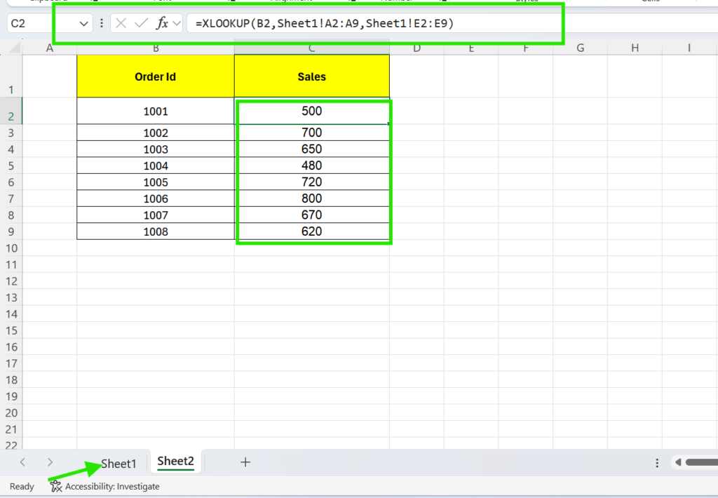
Retrieve sales values from another worksheet dynamically
Formula Used:
=XLOOKUP(B2, Sheet1!A2:A9, Sheet1!E2:E9)
This formula is used to fetch sales data from another sheet based on Order ID. It allows you to link data across sheets dynamically without manual copying.
What This Does
- B2 → Order ID in Sheet2 (input)
- Sheet1!A2:A9 → Order ID column in Sheet1 (lookup range)
- Sheet1!E2:E9 → Sales column in Sheet1 (return range)
How It Works
For example:
Order ID 1001 in Sheet2
→ Excel searches in Sheet1 column A
→ Finds matching row
→ Returns Sales value from Sheet1 column E
👉 Output: 500
This is commonly used in:
- MIS reports
- Multi-sheet dashboards
- Data consolidation files
XLOOKUP with CONCAT (Multiple Conditions)
Sometimes one value isn’t enough to find the correct result. For example, the same Product ID can appear in different regions.
In such cases, we combine (concatenate) two fields – like Product ID + Region – to create a unique lookup value.
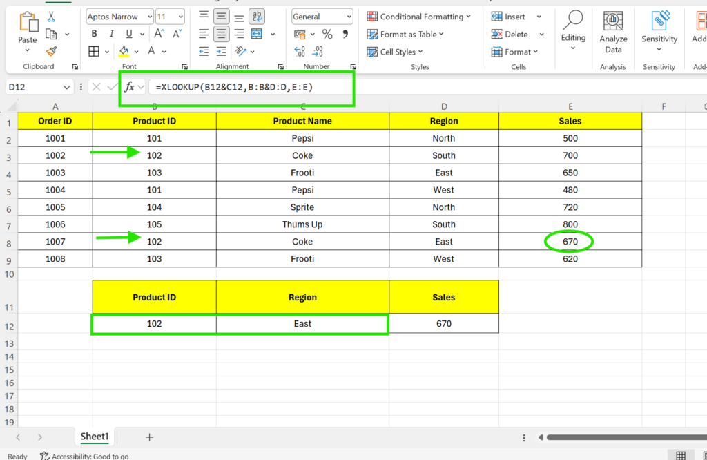
Handle multiple lookup conditions in Excel
Formula Used:
=XLOOKUP(B12&C12, B:B&D:D, E:E)
Explanation:
- B12&C12 → combines Product ID + Region
- B:B&D:D → creates combined lookup column
- E:E → returns Sales
In this example, Product ID 102 appears multiple times in the table:
- Once for South → Sales = 700
- Once for East → Sales = 670
So if you use only Product ID, Excel won’t know which one to pick.
To get the correct result, we add a second condition (Region).
Now instead of searching only by Product ID, we search by:
Product ID + Region
Use multiple conditions in XLOOKUP when a single column has duplicate values.
XLOOKUP Returning Multiple Columns
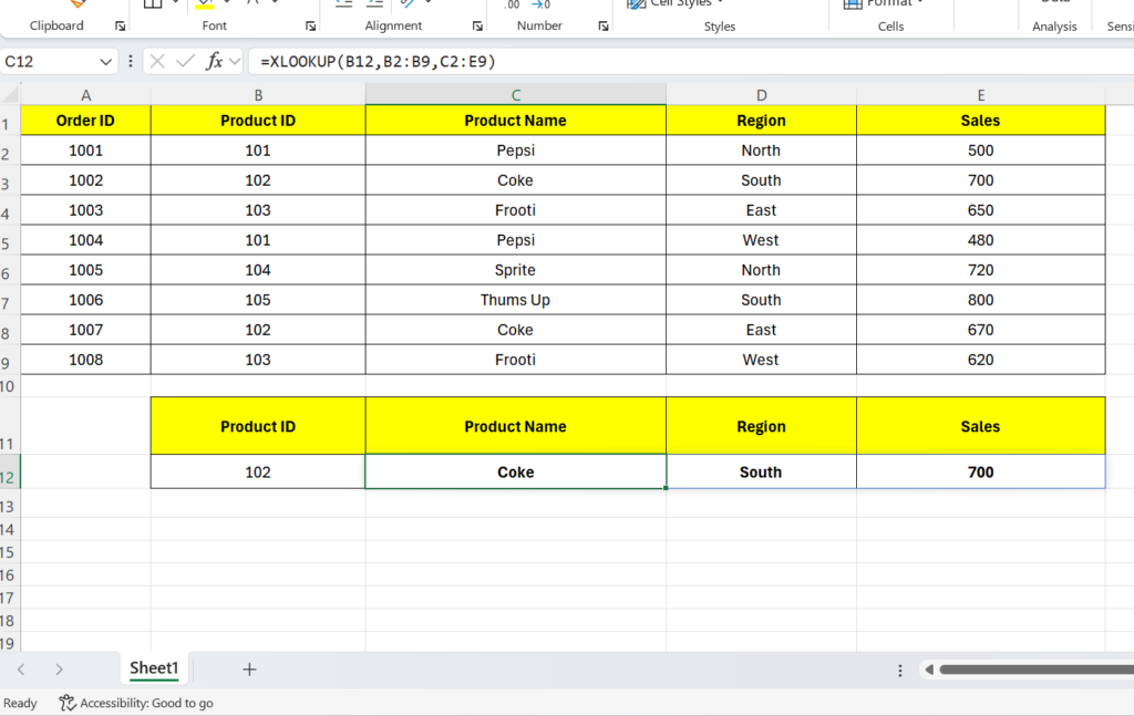
Return multiple columns from a single lookup value
In this example, you are not just fetching one value – you are returning multiple columns at once using this formula.
Formula Used:
=XLOOKUP(B12, B2:B9, C2:E9)
You entered:
- Product ID = 102
Now instead of getting only Sales, you want:
- Product Name
- Region
- Sales
All in one go.
How It Works
- B12 → Lookup value (Product ID = 102)
- B2:B9 → Product ID column (where Excel searches)
- C2:E9 → Multiple columns:
- C → Product Name
- D → Region
- E → Sales
What Happens
Excel:
- Finds 102 in Product ID column
- Moves to that row
- Returns all columns from C to E
If Product ID appears multiple times:
It returns the first matching row only
XLOOKUP + SORT
Use this combinations, when you want to fetch values and then arrange them in order, such as highest sales to lowest sales.
Example formula:
=SORT(XLOOKUP(B2:B9,B2:B9,E2:E9),1,-1)
What this does:
- B2:B9 → Product IDs to search
- B2:B9 → Lookup column
- E2:E9 → Sales column to return
- SORT(…,1,-1) → sorts the returned sales in descending order
Output:
This will return sales like:
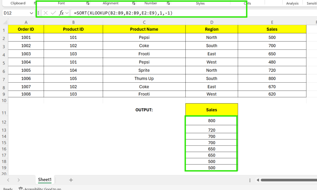
Combining SORT and XLOOKUP formulas to organize sales data dynamically in Excel
This formula first fetches the sales values, and SORT arranges those values from highest to lowest. This is useful when you want to quickly identify top-performing products or create ranking-style reports.
Real Business Use Cases of XLOOKUP
Quickly fetch product-wise sales using SKU/Product ID without manual searching.
Automatically pull data into dashboards for daily and weekly reporting.
Retrieve employee details like salary, department, or performance using Employee ID.
Track stock levels, product availability, and reorder status dynamically.
Fetch latest product prices from master data to avoid manual updates.
XLOOKUP is widely used in modern MIS reporting because it helps combine data from multiple sheets quickly and accurately. You can also read our detailed MIS reporting guide to learn how professionals create structured Excel reports for business teams.
XLOOKUP vs INDEX MATCH
Both XLOOKUP and INDEX MATCH are used to search and return values from a dataset. INDEX MATCH was widely used before XLOOKUP because it was more flexible than VLOOKUP. However, XLOOKUP makes the same task easier, cleaner, and more beginner-friendly.
| Feature | XLOOKUP | INDEX MATCH |
|---|---|---|
| Ease of Use | Easy to understand and write | Slightly complex because it uses two functions together |
| Flexibility | High – works left, right, vertical, and horizontal | High – but requires proper understanding of INDEX and MATCH |
| Learning Curve | Low – beginner-friendly | Medium – needs more practice |
| Error Handling | Built-in error message option | Usually needs IFERROR separately |
| Formula Length | Shorter and cleaner | Longer compared to XLOOKUP |
| Best For | Modern Excel reports, dashboards, and quick lookups | Older Excel versions or advanced legacy files |
XLOOKUP vs VLOOKUP
VLOOKUP was one of the most commonly used lookup functions in older Excel versions. However, XLOOKUP was introduced as a more powerful and flexible replacement with simpler syntax and advanced capabilities.
| Feature | XLOOKUP | VLOOKUP |
|---|---|---|
| Lookup Direction | Can search both left and right | Can only search from left to right |
| Column Index Number | Not required | Required manually |
| Error Handling | Built-in error handling option | Needs IFERROR separately |
| Formula Simplicity | Cleaner and easier to understand | Can become confusing in large datasets |
| Column Insertion Safety | Safe even if columns are added or moved | Can break when columns change |
| Best Use Case | Modern dashboards and reporting | Older Excel files and legacy reports |
Why Modern Excel Users Prefer XLOOKUP
- Works both left and right unlike VLOOKUP
- No column number counting required
- Built-in error handling available
- Safer and easier for beginners
- Supports exact and approximate match
- Works smoothly with dynamic Excel reports
- Perfect for dashboards and MIS reports
- Reduces formula mistakes in large datasets
Common Mistakes While Using XLOOKUP
While XLOOKUP is easy to use, small mistakes in references or ranges can still create incorrect results. Here are some common problems beginners face:
- Using Different Range Sizes: Lookup and return ranges should contain the same number of rows.
- Searching the Wrong Column: Selecting the wrong lookup column can return incorrect values.
- Duplicate Values: XLOOKUP returns the first matching result when duplicates exist.
- Mixing Text and Numbers: Text-formatted values may not match correctly with numeric values.
- No Error Handling: Missing values can show errors if the optional if_not_found argument is not used.
- Using Full Columns: Using entire columns in very large files can reduce workbook performance.
Practice with Dataset
To understand XLOOKUP properly, don’t just read formulas – practice them with a real dataset. Use the dataset below and try solving these questions step by step.
📥 Download Practice Dataset
Download the sample Excel file and practice XLOOKUP formulas using sales data, product IDs, regions, and order details.
Download Dataset🔥 Practice Questions
- Find Sales using Product ID.
- Fetch Product Name dynamically using XLOOKUP.
- Categorize sales as High Sales or Low Sales using IF + XLOOKUP.
- Combine two product sales using SUM + XLOOKUP.
- Find the highest selling product using XLOOKUP logic.
- Fetch sales data from another sheet using XLOOKUP.
If you want practical learning experience, explore our Real Data Lab projects where we work on real Excel datasets, reporting dashboards, and business analysis examples.
Skills You Build While Practicing Excel Formulas
You learn how to connect datasets, identify relationships, and extract meaningful business insights.
Automated formulas reduce manual mistakes and improve report consistency.
These techniques help build dynamic dashboards used in sales, finance, and MIS reporting.
Pro Tips for Using XLOOKUP Faster
- Always lock lookup ranges using $ symbol.
- Keep lookup values clean without extra spaces.
- Use IFERROR with XLOOKUP for cleaner reports.
- Store lookup tables in separate sheets for better management.
- Avoid duplicate Product IDs in lookup columns.
- Use structured tables instead of normal ranges when possible.
- Combine XLOOKUP with FILTER and SORT for advanced dashboards.
✅ Final Thoughts
XLOOKUP is one of the most powerful Excel formulas for modern reporting and data analysis. Whether you work in MIS, sales reporting, finance, HR, or data analytics, learning XLOOKUP can save hours of manual work.
Instead of depending on old formulas like VLOOKUP or complicated INDEX MATCH combinations, XLOOKUP provides a faster, cleaner, and smarter solution for real business reporting.
If you want to improve your Excel and reporting skills further, you can also explore tutorials available on Microsoft Learn, which offers free learning paths for Excel, Power BI, and data analysis.
When Lookup Formulas May Not Be the Best Option
Although lookup formulas are extremely useful, there are situations where other Excel tools may work better.
- Very large datasets with millions of rows
- Files that already use Power Query automation
- Database-style analysis requiring SQL tools
- Complex dashboard models with multiple relationships
- Reports requiring live cloud-based data refresh
In such scenarios, tools like Power Query, Power Pivot, SQL, or Power BI may provide faster and more scalable solutions.
Frequently Asked Questions
Clear answers to common questions about XLOOKUP, formulas, business reporting, lookup techniques, and modern Excel data analysis workflows.
What is XLOOKUP in Excel?
XLOOKUP in Excel is a modern lookup function used to search and return values from tables, datasets, and reports. It is designed to replace older formulas like VLOOKUP and HLOOKUP with a simpler and more flexible approach.
How to use XLOOKUP in Excel?
To use XLOOKUP, you need a lookup value, lookup array, and return array. The formula searches for a value in one column and returns the matching result from another column automatically.
What is the difference between XLOOKUP and VLOOKUP?
XLOOKUP is more advanced than VLOOKUP because it can search both left and right, supports built-in error handling, and does not require column index numbers. It is faster, cleaner, and easier to maintain in modern Excel reports.
Can XLOOKUP replace VLOOKUP?
Yes, XLOOKUP can replace VLOOKUP in most scenarios. Many Excel professionals now prefer XLOOKUP because it offers more flexibility, improved readability, and better accuracy for reporting and dashboard creation.
How does XLOOKUP work with multiple criteria?
XLOOKUP multiple criteria formulas work by combining two or more lookup conditions together. This is useful for advanced Excel reports where you need to match multiple fields like Product ID and Region simultaneously.
Why is XLOOKUP better than older Excel formulas?
XLOOKUP is considered better because it reduces manual errors, supports exact and approximate matching, improves formula readability, and works perfectly for dashboard reporting, MIS reports, and data analysis projects.
Is XLOOKUP useful for business reporting?
Yes, XLOOKUP is widely used in sales reporting, finance, HR reporting, inventory tracking, and MIS dashboards because it helps fetch accurate information quickly from large datasets.
Can beginners learn XLOOKUP easily?
Yes, beginners can learn XLOOKUP easily because the formula syntax is simpler compared to INDEX MATCH combinations. With regular practice and real datasets, most users can understand XLOOKUP quickly.
Ready to Practice XLOOKUP with Real Data?
Download the practice dataset and try XLOOKUP formulas, lookup examples, error handling, and real reporting tasks step by step.
Download XLOOKUP Practice FilePerfect for Excel learners, MIS executives, and data analysis beginners.